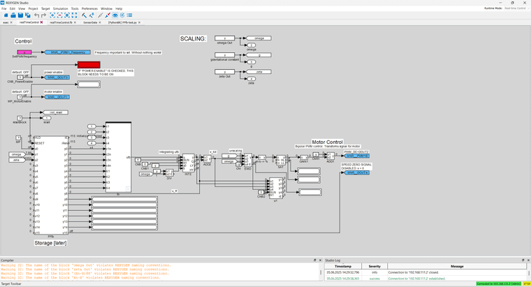
I am not sure how to make the stop in the lower right hand corner run
I am not sure how to make the stop in the lower right hand corner run
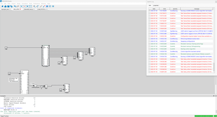
I am not quite sure what this error means or how to fix it if any knows
Hi I am trying to find a way to get my bluetooth sensor(Witmotion WT9011DCL 9-axis BLE Magnetometer Gyroscope) to communiate with rerxygen so I can stream the data into rexygen. I have been able to connect the sensor with my raspberry Pi 4 monacrohat. I then tried to stream the data into rexygen but have been unable to do so. I have attached the my program below. 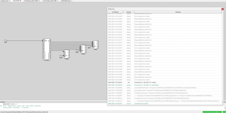
# coding:UTF-8
import asyncio
import bleak
from PyRexExt import REX

class DeviceModel:
    def __init__(self, deviceName, BLEDevice, callback_method):
        self.deviceName = deviceName
        self.BLEDevice = BLEDevice
        self.client = None
        self.writer_characteristic = None
        self.isOpen = False
        self.callback_method = callback_method
        self.TempBytes = []

    async def openDevice(self):
        try:
            async with bleak.BleakClient(self.BLEDevice, timeout=15) as client:
                self.client = client
                self.isOpen = True
                print("Device connected.")
                REX.y9.v = 1  # Connected

                target_service_uuid = "0000ffe5-0000-1000-8000-00805f9a34fb"
                target_characteristic_uuid_read = "0000ffe4-0000-1000-8000-00805f9a34fb"
                target_characteristic_uuid_write = "0000ffe9-0000-1000-8000-00805f9a34fb"
                notify_characteristic = None

                for service in client.services:
                    if service.uuid == target_service_uuid:
                        for char in service.characteristics:
                            if char.uuid == target_characteristic_uuid_read:
                                notify_characteristic = char
                            if char.uuid == target_characteristic_uuid_write:
                                self.writer_characteristic = char

                if self.writer_characteristic:
                    await self.sendData([0xFF, 0xAA, 0x24, 0x01, 0x00])  # 6-axis mode
                    await self.sendData([0xFF, 0xAA, 0x03, 0x09, 0x00])  # 100 Hz

                if notify_characteristic:
                    await client.start_notify(notify_characteristic.uuid, self.onDataReceived)
                    while self.isOpen:
                        await asyncio.sleep(1)
                    await client.stop_notify(notify_characteristic.uuid)
                else:
                    print("Notify characteristic not found.")
                    REX.y9.v = 2  # Failed

        except Exception as e:
            print("BLE connection failed:", e)
            REX.y9.v = 2  # Failed

    def onDataReceived(self, sender, data):
        bytes_list = list(data)
        self.TempBytes.extend(bytes_list)
        if len(self.TempBytes) >= 20:
            if self.TempBytes[0] == 0x55 and self.TempBytes[1] == 0x61:
                self.processData(self.TempBytes[:20])
            self.TempBytes = []

    def processData(self, Bytes):
        def get_val(low, high, scale):
            raw = (high << 8) | low
            val = raw - 65536 if raw >= 32768 else raw
            return round(val / 32768 * scale, 3)

        acc_x = get_val(Bytes[2], Bytes[3], 16)
        acc_y = get_val(Bytes[4], Bytes[5], 16)
        acc_z = get_val(Bytes[6], Bytes[7], 16)
        gyro_x = get_val(Bytes[8], Bytes[9], 2000)
        gyro_y = get_val(Bytes[10], Bytes[11], 2000)
        gyro_z = get_val(Bytes[12], Bytes[13], 2000)
        ang_x = get_val(Bytes[14], Bytes[15], 180)
        ang_y = get_val(Bytes[16], Bytes[17], 180)
        ang_z = get_val(Bytes[18], Bytes[19], 180)

        # Send to REXYGEN outputs
        REX.y0.v = acc_x
        REX.y1.v = acc_y
        REX.y2.v = acc_z
        REX.y3.v = gyro_x
        REX.y4.v = gyro_y
        REX.y5.v = gyro_z
        REX.y6.v = ang_x
        REX.y7.v = ang_y
        REX.y8.v = ang_z

        print("Data:", acc_x, acc_y, acc_z, gyro_x, gyro_y, gyro_z, ang_x, ang_y, ang_z)

    async def sendData(self, data):
        try:
            if self.client and self.writer_characteristic:
                await self.client.write_gatt_char(self.writer_characteristic.uuid, bytes(data))
        except Exception as e:
            print("Write failed:", e)

class BLEScanner:
    def __init__(self, target_mac="CC:0E:4F:3B:A4:3B"):
        self.target_mac = target_mac
        self.BLEDevice = None
        self.device_model = None

    async def scan_and_connect(self):
        try:
            print("Scanning for BLE devices...")
            devices = await bleak.BleakScanner.discover(timeout=10.0)
            for d in devices:
                if d.address == self.target_mac:
                    self.BLEDevice = d
                    break

            if not self.BLEDevice:
                print("Target device not found.")
                REX.y9.v = 2
                return

            self.device_model = DeviceModel("MyBLE", self.BLEDevice, None)
            await self.device_model.openDevice()

        except Exception as e:
            print("Scan or connect error:", e)
            REX.y9.v = 2

def run_ble_task():
    loop = asyncio.new_event_loop()
    asyncio.set_event_loop(loop)
    scanner = BLEScanner()
    loop.run_until_complete(scanner.scan_and_connect())
    loop.close()

# Main entry point for REXYGEN
if __name__ == "__main__":
    print("Starting REXYGEN BLE program")
    REX.y9.v = 2  # Default = failed
    run_ble_task()
Hi I am trying to connect my bluetooth sensor(Witmotion WT9011DCL 9-axis BLE Magnetometer Gyroscope) to rexygen via bluetooth so I can stream the data from the sensor into rexygen. I am not sure how to get started on this.
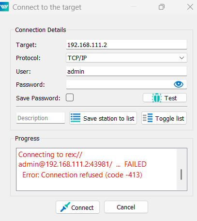
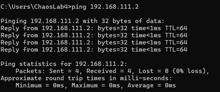
I am unable to conneect to the rexygen to my Raspberry Pi.
@cechurat Hi Thomas when I hover my mouse over the error I get this message.
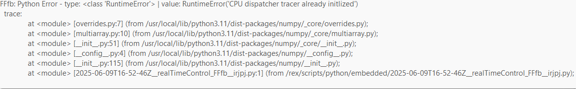
I am not quite sure what it means or how to fix it
@cechurat 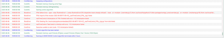
I think the problem might be in the python block.
import numpy as np
import time
from numpy import sin,cos,pi
from scipy.integrate import solve_ivp, solve_bvp, quad, odeint
from scipy.linalg import solve_continuous_are
from scipy.interpolate import interp1d
#import matplotlib.pyplot as plt
from PyRexExt import REX
def init():
global ω,ζ,π,τ,τ1,τpred,xmax,umax,θinti,θdotinit,xinit,xdotinit,xstate_init,θend1,θend2,θdotend,xend,xdotend,xstate_end1,xstate_end2,Q,R,ts,dt,ts1,bvpfcn,bcfcn,ff,uff0,uff,runningCost,A,B,mRiccati,Sall,Ball,Kall,fpred,us,j
global xstate_end,FFsol,X,uff,vs,Kvec,Xlast,Klast
############################################ Define parameters
ω          = REX.u1.v
ζ          = REX.u2.v;                      # pendulum friction (scaled: 1 = critical damping)
π          = pi;                            # π = 3.14159...
τ          = 2*π                            # swingup time = 1 period, in scaled units
τpred      = 1                              # allow for calculation time, in scaled units
τ1         = 2*τ                            # for sim: swingup + balance time
xmax       = 2;                             # track limits at ±xmax
umax       = 5;                             # clip u for simulation test ONLY (not design)

θinit      = 0;                             # initial angle of pendulum
θdotinit   = 0.0;                           # initial angular velocity of pendulum
xinit      = 0.0;                           # initial position of cart
xdotinit   = 0.0;                           # initial velocity of cart
xstate_init = np.array([θinit,θdotinit,xinit,xdotinit])        # eventually, from expt.

θend1      = π                              # CCW swingup,   assume θinit ∊ (-π,π)
θend2      = -π                             # CW swingup
θdotend    = 0.0;                           # final angular velocity of pendulum
xend       = 0.0 * xmax;                    # final cart position
xdotend    = 0.0;                           # final cart velocity
xstate_end1 = np.array([θend1,θdotend,xend,xdotend])   # modify for swing down, transport, ...
xstate_end2 = np.array([θend2,θdotend,xend,xdotend])   # modify for swing down, transport, ...

Q    = np.diag([1,10,1,1])                  # weighting for states for LQR
R    = np.array([10])                       # weighting for input for LQR

ts   = np.arange(0, τ, 0.01*ω)       # swing up in τ
dt   = 0.01*ω
ts1  = np.arange(0, τ1, 0.01*ω)      # swing up in τ, balance for another τ

############################################# Define functions
def bvpfcn(t, X):                           # solve coupled state-adjoint system

    θ, θdot, x, xdot, λθ, λθdot, λx, λxdot = X

    dX = np.zeros((8, X.shape[1]))          # array dimension is 8 * nx
    sinθ = sin(θ);  cosθ = cos(θ)

    u = -λxdot + λθdot*cosθ

    dX[0] = θdot
    dX[1] = -sinθ - u*cosθ
    dX[2] = xdot
    dX[3] = u

    dX[4] = λθdot * (cosθ - u*sinθ)
    dX[5] = - λθ
    # dX[6] = -x**3 / xmax**4                 # or:  from running cost term (x/xmax)**4
    dX[6] = 0                               # running cost independent of x
    dX[7] = -λx

    return dX                               # Return derivatives (array)

def bcfcn(x0, xτ):                          # boundary conditions for 4d-state at t = 0, τ
    dx0 = x0[0:4] - xstate_init             # boundary condition for 4d state at t=0
    dxτ = xτ[0:4] - xstate_end              # bc                              at t=τ
    return np.hstack((dx0,dxτ))             # 8-dim vector for solve_bvp

def ff(x0,xτ,τ):                            # ff state x0 → xτ in τ
    θinit,_,xinit,_ = x0
    θend, _,xend, _ = xτ

    nt = 21                                            # number of time points, to start
    tvec = np.linspace(0, τ, nt)
    xλguess = np.zeros((8, nt))                        # initial guesses for state trajectories
    xλguess[0, :] = np.linspace(θinit, θend, num=nt)   # θ linear, θinit → θend
    xλguess[2, :] = np.linspace(xinit, xend, num=nt)   # x linear, xinit → xend

    FFsol = solve_bvp(bvpfcn, bcfcn, tvec, xλguess, tol=0.1)   # solve boundary-value problem
    return FFsol.sol

def uff0(t):                                # feedforward acceleration (cannot evaluate on arrays)
    θ,_,_,_,_,λθdot,_,λxdot = FFsol(t)      # evaluate interp funcs at time=t
    uff0 = -λxdot + λθdot*cos(θ) if t<τ else 0
    return uff0
uff = np.vectorize(uff0)                    # define vectorized version (can call with array)

def runningCost(t):                         # to calc cost of the feedforward command
    return 0.5*uff0(t)**2

def A(t):                                   # dynamical matrix (local linear, nominal)
    θ         = FFsol(t)[0]                 # FFsol from FF function
    Amat      = np.zeros((4,4))             # 4 is from xstate.shape[0]
    Amat[0,1] = 1
    Amat[1,0] = -cos(θ) + uff(t)*sin(θ)
    Amat[1,1] = 0
    Amat[2,3] = 1
    return Amat                             # evaluated at time t

def B(t):                                   # input vector (local linear, nominal)
    θ       = FFsol(t)[0]                   # FFsol from FF function
    Bmat    = np.zeros((4,1))               # 4 is from xstate.shape[0]
    Bmat[1] = -cos(θ)
    Bmat[3] = 1
    return Bmat

def mRiccati(t,S):                          # derivatives for matrix Riccati (vector form)
    Smat = S.reshape((4,4))                 # convert 16 vector to 4x4 matrix
    A0 = A(t)                               # current dynamical matrix
    B0 = B(t)                               # current input vector
    dSmat = - A0.T @ Smat - Smat @ A0 - Q + Smat @ (B0 @ B0.T) @ Smat / R[0]
    dS = dSmat.reshape((16))                # convert 4x4 matrix to 16 vector
    return dS

def Sall(Send,τ,tvec):                      # S matrix evaluated at times tvec
    Send1 = Send.reshape((16))
    t_span = (τ, 0)                         # solve backwards in time, from τ → 0
    Ssol1 = solve_ivp(mRiccati, t_span, Send1, dense_output=True).sol
    return Ssol1(tvec).reshape(4,4,tvec.size)   # evaluate on tvec

def Ball(FFsol,tvec):                       # input matrix (local linear, nominal)
    θ       = FFsol(tvec)[0]
    nt      = tvec.size
    Bmat    = np.zeros((4,nt))              # 4 is from xstate.shape[0]
    Bmat[1] = -cos(θ)
    Bmat[3] = np.ones((nt))
    return Bmat

def Kall(Send,FFsol,τ,tvec):                # for graphing
    tvec1 = np.clip(tvec, 0, τ)             # elements beyond ff range are clipped to limits
    S = Sall(Send,τ,tvec1)                  # 4 x 4 x nt matrix (nt copies of 4x4 matrix
    B = Ball(FFsol,tvec1)                   # 4 x nt matrix     (nt copies of 4-vector)
    return np.einsum('ijk,jk->ik', S, B)/R[0]   # sum over inner index, element-mult tvec index

def fpred(t,xstate):                        # dynamical eqs, for constant-v input
    θ, θdot, _, xdot = xstate               # dynamical states
    dX = np.zeros((4))                      # 4 is from xstate.shape[0]
    dX[0] = θdot
    dX[1] = -sin(θ) - 2*ζ*θdot              # sim has pendulum friction, even if ff does not
    dX[2] = xdot
    dX[3] = 0                               # driving term is vtot; utot is a derived variable
    return dX

############################################# prediction of future state
xpred  = solve_ivp(fpred, (0, τpred), xstate_init, dense_output=True).sol # predict future state
xstate_init  = xpred(τpred)                 # "initial" state, as predicted τpred in future
θ0 = xstate_init[0];                        # extrapolated θ0 might not be ∊ (-π,π)
θ1 = (θ0+π) % (2*π) - π                     # modulus 2π
xstate_init[0] = θ1                         # new angle is ∊ (-π,π)

############################################# FF calculations
xstate_end = xstate_end1; θend = θend1
FFsol  = ff(xstate_init,xstate_end,τ)       # ff solution for 4-state and 4-adjoint, 0→τ
FFsol1 = FFsol
Jff1   = 0.5*np.sum(uff(ts)**2)*dt          # integrated running cost = overall cost

xstate_end = xstate_end2; θend = θend2
FFsol  = ff(xstate_init,xstate_end,τ)       # ff solution for 4-state and 4-adjoint, 0→τ
FFsol2 = FFsol
Jff2   = 0.5*np.sum(uff(ts)**2)*dt          # integrated running cost = overall cost
REX.y11.v = f"feedforward cost: θend = π, Jff1 = {Jff1:0.2f}, θend = -π, Jff2 = {Jff2:0.2f}"

if (Jff1 < Jff2):
    FFsol = FFsol1;   xstate_end = xstate_end1
else:
    FFsol = FFsol2;   xstate_end = xstate_end2

############################################### fb calculations
Aend = A(τ)                                   # linear dynamics A matrix at t=τ
Bend = B(τ)                                   # linear input-coupling B vector at t=τ
Send = solve_continuous_are(Aend,Bend,Q,R)    # static S matrix from ARE
Kvec = Kall(Send,FFsol,τ,ts1)                 # feedback gain vectors for t in ts1

############################################### get arrays
θs,θdot,x, xdot,_,_,_,_ = FFsol(ts)
X = np.array([θs,θdot,x,xdot])

θlast,θdotlast,xlast,xdotlast,_,_,_,_=FFsol(2*π)                # Evaluate last values
Xlast   = np.array([[θlast],[θdotlast],[xlast],[xdotlast]])
X       = np.hstack((X,Xlast))                                  # add last value

Klast   = Kall(Send,FFsol,τ,2*π+0.1)
Kvec    = np.hstack((Kvec,Klast))

vs      = np.hstack((xdot,0))
j=0
def main():
start_test = time.perf_counter()
global j,X,uff,vs,Kvec
if not REX.u0.v and j == 0:
    return
else: REX.y15.v = True

REX.y10.v= f"len(X)={len(X[0])}"
if (j >= len(X[0])):
    REX.y8.v = 0
    return

# Value for every time
REX.y0.v = X[0][j]
REX.y1.v = X[1][j]
REX.y2.v = X[2][j]
REX.y3.v = X[3][j]
REX.y4.v = Kvec[0][j]
REX.y5.v = Kvec[1][j]
REX.y6.v = Kvec[2][j]
REX.y7.v = Kvec[3][j]
REX.y8.v = vs[j]
j += 1

test_time = time.perf_counter() - start_test
REX.y9.v = f"test time = {test_time:0.3f} s"

return
def exit():
# PUT YOUR CODE HERE
return
I am not sure how to make the stop in the lower right hand corner run