EKF example
-
I would like to use the EKF (extended Kalman filter) block. I have seen a very complicated example via my colleague, but it has too many extraneous parts to be understandable.
Our case is very simple. To give the simplest form, consider a pendulum, theta''[t] + sin[theta] = u[t], where u is a deterministic (known) input signal. We measure theta[t] (has noise) and want to estimate the velocity theta'[t] via the EKF. The measurements are rapid enough, relative to the period, that a simple discrete time EKF (e.g. Euler step) should be fine. So no fancy integration techniques are needed.
Does someone know how to set up such an example for the EKF block (or have something equivalent)? That would help us a lot. Thanks!
-
@bech Hi,
I'm sending an example of using EKF for a linear model. Please take a look at the code in the REXLANG block. Unfortunately, I don't have time to document the example in more detail right now. However, I should have time next week, so I'll send an improved version then.
Best regards,
Jan
EKF.zip -
@Jan-Reitinger Thank you. We are in the process of trying to understand the example better and to start to modify for our case. Any documentation or comments on the supplied example that you have time for would be welcome.
-
@bech Hi,
here is a Markdown file describing the system, which is implemented in the REXLANG block. To view the equations correctly, copy the file's contents into an online editor, such as this one: https://markdownlivepreview.org -
EKF - Linear System Model
This document describes the use of the Extended Kalman Filter (EKF) in the REXYGEN environment for state estimation of a linear system.
System Description
The system is described by the following differential equations:
\begin{aligned}
\frac{dx(t)}{dt} &= f(x(t), u(t)) + w(t),\\
y(t) &= h(x(t), u(t)) + v(t),\\
\hat{x}(t) &\sim \mathcal{N}(x, P),\\
w(t) &\sim \mathcal{N}(0, Q),\\
v(t) &\sim \mathcal{N}(0, R).
\end{aligned}
where:
- $ x(t) $ is the state vector,
- $ u(t) $ is the input vector,
- $ y(t) $ is the output vector,
- $ w(t) $ is the process noise,
- $ v(t) $ is the measurement noise,
- $ \hat{x}(t) $ is the estimated state vector,
- $ x $ is the mean (expected value),
- $ P $ is the state estimation covariance matrix,
- $ Q $ is the process noise covariance matrix,
- $ R $ is the measurement noise covariance matrix.
State Model of the System
The system dynamics are defined by the function $ f(x(t), u(t)) $:
f(x(t), u(t)) =
\begin{bmatrix}
\frac{dx_1(t)}{dt} \\
\frac{dx_2(t)}{dt} \\
\frac{dx_3(t)}{dt} \\
\frac{dx_4(t)}{dt}
\end{bmatrix}
=
\begin{bmatrix}
-x_1(t) + x_2(t) \\
-x_2(t) + x_3(t) \\
-x_3(t) + x_4(t) \\
-x_4(t) + u_1(t)
\end{bmatrix}.
Jacobian of the State Function
The Jacobian $ f(x, u) $ with respect to the state vector $ x $ is given as:
\frac{df(x(t), u(t))}{dx} =
\begin{bmatrix}
-1 & 1 & 0 & 0 \\
0 & -1 & 1 & 0 \\
0 & 0 & -1 & 1 \\
0 & 0 & 0 & -1
\end{bmatrix}
Output Measurements
The first set of output measurements (which, in this example, depend linearly on the state variables) for input EKF:nz = 1 is defined as:
y(t) = h_1(x(t), u(t)) =
\begin{bmatrix}
x_1(t) \\
2 x_2(t) + 0.5 x_4(t)
\end{bmatrix},
with the corresponding Jacobian:
\frac{dh_1(x(t), u(t))}{dt} =
\begin{bmatrix}
1 & 0 & 0 & 0 \\
0 & 2 & 0 & 0.5 \\
\end{bmatrix}.
The second set of output measurements (for input EKF:nz = 2) is not used.
The system description is programmed into the REXLANG block.
This description serves as a basis for implementing the EKF in REXYGEN using the EKF function block. Further details can be found in the official documentation: EKF Block in REXYGEN.
-
@Jan-Reitinger I upgraded your example. Now it uses exact reference model both for verification and emulating output measurements to be used as input to the estimator.
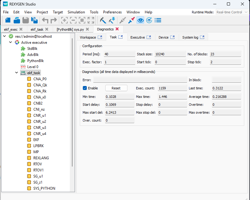
However, there is some timing issue here. I use tick=0.02, ntick0=4. It means period of the task is 80 ms. If I go lower with that, I receive overtime in diagnostics. This is odd, because it means that computational load is too high.
It should be much less than that.
Here is my current version:
EKF_John.zip -
@stepan-ozana
First of all, thank you very much for adding the reference model. If you agree, I would like to add this model to the example on EKF, which is already part of the daily version of REXYGEN.As for the timing. I think the problem may be in the Python block, which takes significantly longer to execute than the native blocks. Try looking in the Diagnostics and at the statistics on the execution of the task.
-
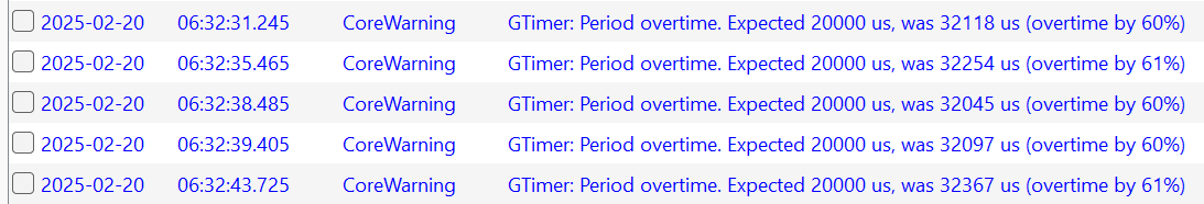
@Jan-Reitinger Sure! I'm glad to have contributed to the collection of examples. Regarding the timing issue, I may have used the wrong terminology. I don’t observe 'Overtime' in the Task Diagnostics, but I do see 'CoreWarning GTimer: Period overtime.' in the System log.
This issue occurs in the original 'EKF.zip' mentioned at the beginning of this thread—at least on my PC. It may function correctly on other machines. It may be due to using Windows instead of Linux. I will tes it on Linux.
Here is the screenshot:
Moreover:
I just realized that the current version of the example is not fully correct because it lacks process noise and measurement noise. It seems that process noise should be implemented within the block currently referred to as the 'Reference Exact Model,' which would no longer be 'exact.' Measurement noise can be simply introduced as an added signal to the model's output.I will try to incorporate these modifications in the next few days. I plan to create a 'Reference Model' that mimics the real process while accounting for both types of noise. Once I have refined the example to meet my expectations, I will get back to you.
-
@stepan-ozana Thank you for your valuable insights! Your contribution to the collection of examples is greatly appreciated.
In the original 'EKF.zip' file mentioned at the beginning of this thread, the timing parameters were incorrectly set—my apologies for that. The best way to correct them is by changing the start and stop values in the task1 block to -1, as outlined in the manual. The log message 'CoreWarning GTimer: Period overtime.' appears whenever the task execution exceeds the maximum allowed time, which can be observed in Diagnostics. If this warning appears in the log while the Max time in Diagnostics does not exceed the allocated execution time (20 ms in the case of EKF.zip), it indicates an error.
We would greatly appreciate any further insights and improvements from your side. I had planned to simulate measurement noise similarly to your approach—by adding white noise to the measurement vector—but I hadn’t considered process noise. For your reference, I’m sharing the updated version of the example, which includes your reference model and the corrected timing parameters.
-
@Jan-Reitinger I suggest having both "reference model" suffering from noises and "reference exact model" for comparison of EKF efficiency and performance.
Please take a look at my suggestions and let me know your opinion. It seems to work. Maybe it needs a bit tuning in terms of Q,R, versus noise generators. Also, I am fighting with alignment of free text within boxes.
Here is my update:
linear-system_v2.zip -
@stepan-ozana
Thanks, that looks great! I'll modify the schema a little more to match the conventions of the other blocks and include it in the installation. -
@Jan-Reitinger Nice. Just one small remark: There's no need to use a two-dimensional input here—even formally. You can define a system with a one-dimensional input, a certain number of states, and possibly a different number of outputs. Instead of using u(t)=[sin(2πt);0] you can simply write u=u1=sin(2πt).